
Maybe creating new municipalities was a good idea...
That doesn't mean Brazil needs more municipalities.


Disclaimer: Claude was used for the illustration on the splits, as my design skills are subpar
A new working paper by Dahis and Szerman (2025) documents what happened when Brazil added 1,383 new municipalities in eight years. The results push back against the standard fiscal critique of decentralization, without quite settling whether the country should have done more of it.
The textbook debate about decentralization assumes the political units already exist, and the only question is how much power to push down to them. That is the world of Wallace Oates writing about American federalism (Oates, 1972), of Charles Tiebout sketching his suburban voters (Tiebout, 1956). Step into most of the developing world and the prior question becomes inescapable: how many local governments should there be?
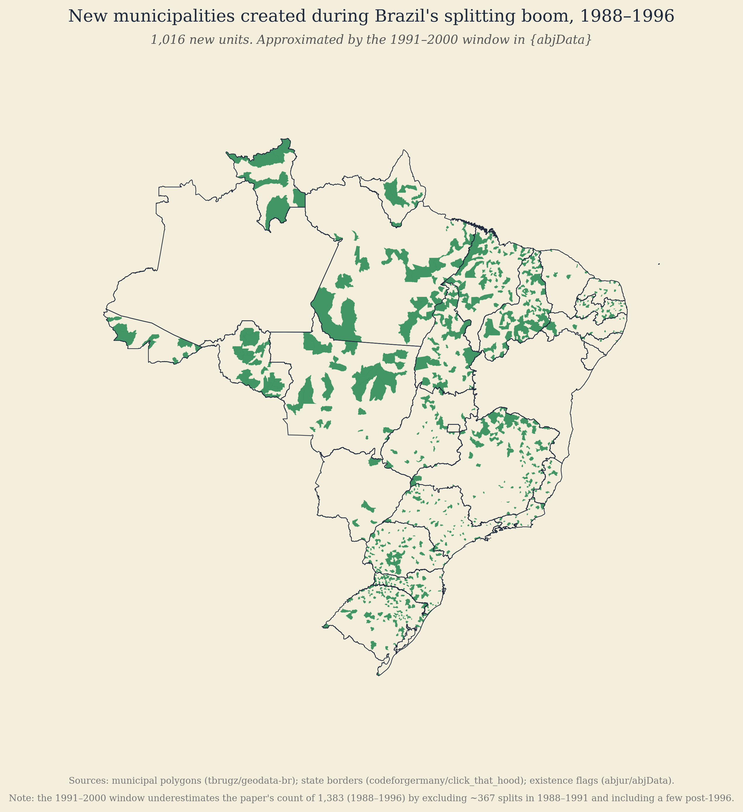
Brazil ran an unusually clean version of that experiment between 1988 and 1996. Coming out of military rule, the new constitution made municipalities into real governments. They collect taxes, run schools, deliver services, and elect their own mayors. It also handed states the authority to write their own rules for creating new municipalities, and most states wrote permissive ones. Small towns and rural districts started petitioning to leave their parent municipalities, and the state legislatures said yes. As per the new constitution, federal transfers kicked in for the new units, which incentivised new polities to emerge. Over the next eight years, Brazil added 1,383 new municipalities, a 34% expansion of the country’s political map.
To anyone trained in the canon of fiscal federalism, the obvious worry was overreach. More units mean more bureaucracies, more demand on shared transfers, and more openings for narrow interests to capture small governments that lack the scale to deliver. Alesina and Spolaore (1997) and Boffa, Piolatto, and Ponzetto (2016) laid out the case carefully. Smaller jurisdictions forgo economies of scale and survive only because the rest of the country subsidizes them. By 1996, the Brazilian Congress had heard enough and approved a constitutional amendment to shut the process down.
That window is what Dahis and Szerman (2025) work with. Armed with decades of follow-up data on municipalities, such as fine-grained fiscal records, matched employer-employee files, satellite night lights… they studied Brazil during the boom as one of the better-instrumented natural experiments in the decentralization literature… Well, guess what? Turns out the warnings may have been misguided.
The political economy behind the boom of new municipalities
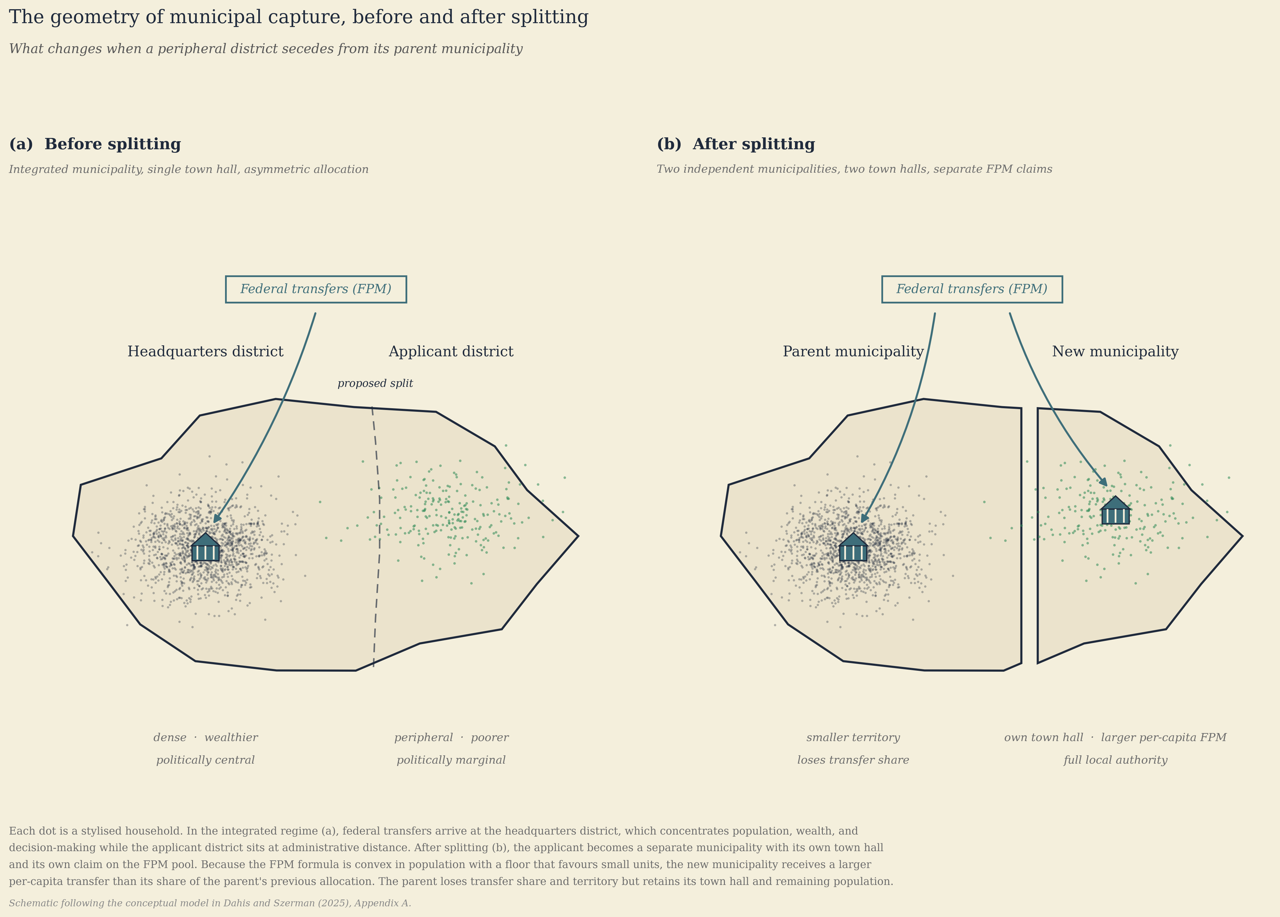
The mechanism that turned permissive rules into a thousand-plus new municipalities was the Fundo de Participação dos Municípios. The FPM is the federal transfer that supplies between thirty and 60% of revenue for the typical Brazilian municipality, and the way it is allocated did most of the heavy lifting.
Each year, 22.5% of federal revenues from income tax and the industrial product tax flow into the FPM pool. The pool is divided by state into block grants, and within each state, municipalities receive shares according to a convex step-wise formula on population. The formula has a floor that disproportionately benefits municipalities below roughly 10,188 inhabitants (Tomio, 2002). A small new municipality of, say, 8,000 people gets a per-capita transfer well above what an established municipality of 50,000 receives. The fund is zero-sum within each state. When a new municipality is created, the state block grant gets resliced, and the existing municipalities each lose a sliver of their previous share.
This generates an obvious arbitrage. If a peripheral district with 8,000 residents splits off from a parent municipality of 100,000, the new municipality moves from a per-capita FPM share calculated on the parent’s bracket to its own much higher per-capita share calculated on its own bracket. The total state-level transfer pool does not change. The redistribution from older to newer municipalities is built into the formula.
Layered on top of this, 15% of FPM transfers are earmarked for education and 15% for health (Brollo, Nannicini, Perotti, and Tabellini, 2013). The rest are unmarked. Local taxation and fees average around five percent of total municipal revenues. The decentralized Brazilian municipality is, on the revenue side, mostly a vehicle for spending federal transfers.
The decision to split also responded to non-fiscal pressures. A 1993 survey of Brazilian mayors found that the two most common reasons given for seeking emancipation were neglect by the parent local government (63%) and the territorial size of the original municipality (24%) (Bremaeker, 1993). The districts that wanted out were peripheral, poorer than their parent municipalities, more remote from the old town hall, and politically marginalized by the elites in the denser headquarters of the municipalities.
Before going to the empirical work it is worth taking a closer look on the conceptual model the authors sketch in their appendix, because it disciplines the empirical predictions and clarifies what each result is and is not testing.
The setup is a minimal Tiebout-style framework in the tradition of Bolton and Roland (1997) and Dur and Staal (2008). Imagine a municipality made of two districts, A and B, where A holds the headquarters and decision-making authority. The headquarters chooses public-goods provision across both districts by maximizing a Pareto-weighted sum of utilities, with weight λ on district B and (1 − λ) on district A. Lower λ means more capture and neglect of the periphery by the headquarters. Revenues come from a uniform income tax τ and from federal transfers T(·), where T is weakly increasing and concave in population. Concavity is the FPM floor logic in shorthand.
In the integrated regime, the headquarters chooses public goods in A and B and a tax rate. In the split regime, district B chooses its own provision and tax rate, subject to a smaller transfer T(αB). Comparing solutions yields two predictions worth singling out. First, the benefits of splitting for the seceding district are larger when it was more captured and neglected by the headquarters (low λ), and when it has a high comparative gain in transfers if split. Second, conditional on the rest of the country being much larger than the splitting district and on the splitter being small and neglected, the welfare change for the parent district is small, the welfare gain for the seceding district is large, and the welfare loss for the rest of the country is small.
The model gives the empirical work three targets. Splitting should benefit the applicants most when they look neglected and peripheral at baseline, the parent headquarters should not see much, and the rest of the country should not see much either. The empirical results confirm all three hypotheses.
Solving the Selection Problem
The hardest thing about studying municipal splits is that… well, the units choose to split. Whatever drives a district to push for emancipation, poverty, distance, political marginalization, and neglect also shape its economic trajectory. Comparing splits to non-splits just gives you back the underlying selection.
Dahis and Szerman (2025) get around this by going to the state archives. Between 1988 and 1996, every district that wanted to split had to file a formal petition, win a local referendum, and get past the state legislature. Plenty of petitions failed: vetoed by committees, blocked by governors, defeated in referenda, left pending when the 1996 amendment hit. The authors hand-collected eleven states’ worth of these records and built a control group of “almost-split” districts. Places that wanted out, started the process, and got stopped for reasons unrelated to their economic prospects.
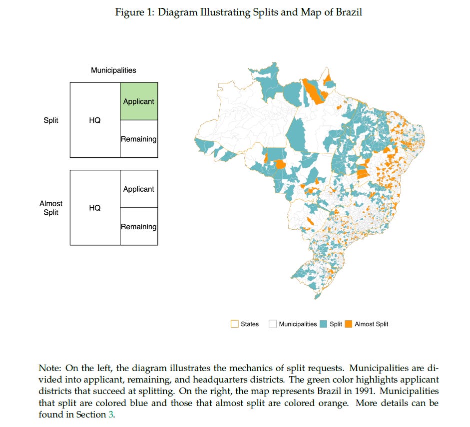
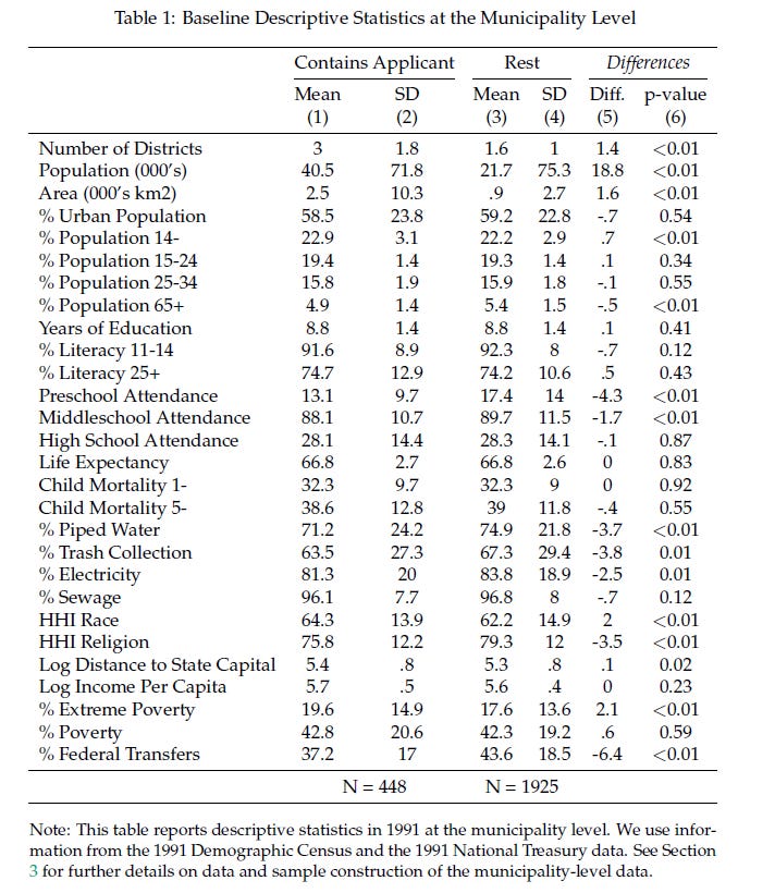
That is the identification strategy. It works because the failed petitions look a lot like the successful ones statistically (Table 1). Both come from poorer-than-average municipalities, both are larger and more rural, and both feel the same federal transfer formula. The only thing that separates them is essentially procedural luck.
The empirical model is a difference-in-differences specification estimated on two waves of splits, in 1993 and 1997. Both waves followed Brazilian municipal election cycles, which is the moment at which newly elected officials in the recently created municipalities took office. The baseline regression in Dahis and Szerman (2025) takes the form
where y_mst denotes the outcome of interest for municipality m in state s in year t, α_m absorbs time-invariant municipality characteristics, α_st captures state-specific shocks in each year, Split_m is an indicator equal to one for municipalities that ultimately split, W_m is the wave-year in which municipality m split (1993 or 1997), and the indicators 1[t − W_m = τ] index event-time relative to the split. The coefficient β_{−1} is normalised to zero, so that the post-event coefficients β_τ trace out the dynamic effect of splitting relative to the year immediately before the wave. Standard errors are two-way clustered at the state and split-wave levels1.
The control group is composed of almost-split municipalities, which contain at least one applicant district whose petition ultimately failed for reasons unrelated to local economic potential. Importantly, these control municipalities are never treated within the sample window. The design, therefore, relies on a clean, never-treated comparison group rather than on a contrast between earlier-treated and later-treated units.
The canonical concerns about two-way fixed effects estimators with staggered treatment, raised by Goodman-Bacon (2021), Callaway and Sant’Anna (2021), Borusyak, Jaravel, and Spiess (2024), de Chaisemartin and D’Haultfœuille (2020), and Sun and Abraham (2021), are mitigated by construction in this setting. Those concerns arise when staggered treatment timing leads earlier-treated units to be used as effective controls for later-treated units, contaminating the estimated average treatment effect under heterogeneous individual effects.
With only two waves of treatment and a stable never-treated control group, the variance decomposition of the difference-in-differences estimator places negligible weight on forbidden comparisons. Robustness exercises reported in the paper re-estimate the principal results separately for the 1993 and 1997 waves and recover quantitatively similar magnitudes, a pattern that would not be expected if the staggered-treatment problem were materially distorting the estimates.
The identifying assumption is that, in the absence of splitting, treated and almost-treated municipalities would have evolved along parallel trajectories. The event-study coefficients β_τ for τ < −1 provide a direct visual test of this assumption. Across the principal outcomes, those pre-event coefficients sit statistically and substantively close to zero, which is the empirical analogue of parallel pre-trends.
Dahis and Szerman (2025) complement the difference-in-differences design with a regression-discontinuity strategy that exploits a distinct source of identifying variation. Before the 1996 constitutional amendment, every district seeking to split was required to obtain at least a simple majority of valid votes in a local referendum. Minas Gerais is the only Brazilian state for which referendum vote shares are publicly reported, but this isn’t a problem as the state is broadly comparable to the rest of the country on dimensions that matter for external validity. Minas Gerais is the second most populous and third wealthiest state in Brazil, with an area larger than that of metropolitan France, and its ethnic composition and geographical features are close to the national averages.
The authors implement a difference-in-discontinuities specification in two stages. The first stage models the probability of splitting as a function of crossing the 50% vote threshold,
where RV_d is the referendum vote share in favour of splitting in district d and g(RV_d) is a linear distance function from the cutoff. The second stage estimates the effect of splitting on outcomes,
with district and year fixed effects, an interaction of the running variable with the post-wave indicator, and a vector X_dt of pre-determined controls. The preferred specification uses a 15% bandwidth around the 50% cutoff in order to balance bias against precision.
The first stage delivers a sharp jump at the threshold: crossing the simple-majority requirement raises the probability of splitting by 0.96, which corresponds to the expected mechanical effect of a binding electoral rule. The reduced-form effect of crossing the threshold on log luminosity for applicant districts is 0.16 and statistically significant at the one-percent level. This implies a Wald estimate of approximately 0.27 (≈ 0.16 / 0.96), or a twenty-eight percent gain in luminosity attributable to splitting, almost identical to the difference-in-differences estimate of 26% obtained when the sample is restricted to Minas Gerais.
The continuity test of pre-referendum characteristics around the threshold is clean for log area, log baseline luminosity, and log distance to the parent town hall. The single exception is log population, which exhibits a modest discontinuity at the cutoff. The authors address this by including interactions of baseline population with year fixed effects, which allow for differential trends by initial population size and absorb the only visible threat to the local exogeneity assumption.
The two designs rest on distinct identifying assumptions. The difference-in-differences strategy relies on parallel counterfactual trends between treated and almost-treated municipalities. The regression-discontinuity strategy relies on continuity of potential outcomes at the 50% vote threshold. No obvious source of confounding would generate parallel violations of both assumptions with comparable magnitudes, which is why the convergence of the two estimators around a twenty-six to 28% luminosity gain is more reassuring than either point estimate considered in isolation.
What Happens When a District Becomes a Municipality?
The first thing it does is build a bureaucracy. Capital expenditures jump by about 40% in the year of the split and settle at 27% above the counterfactual over the next 15 years. Current spending, the payroll and day-to-day operations bucket, rises by 17%. Municipal headcount grows by 16%. Average wages do not budge. New municipalities expand by hiring, not by paying existing workers more.
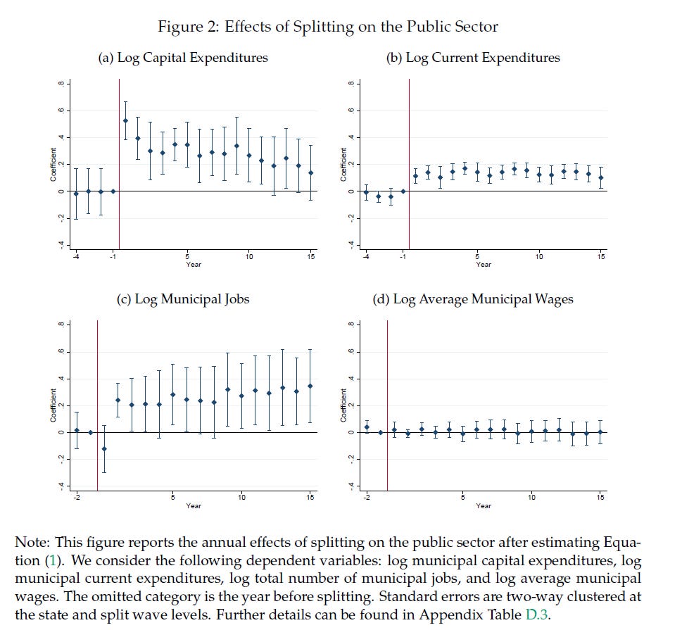
The pattern of capital expenditures rising faster than current expenditures is consistent with the institutional reading. Capital spending captures one-time outlays on machinery, vehicles, and buildings, the basic setup costs of a new local government. Current spending captures the ongoing payroll and operations. The initial jump in capital is a setup burst, and the steady plateau in current spending is the new equilibrium of running a municipality. Lima and Silveira Neto (2018) noted the same broad pattern in earlier work on Brazilian secessions, but without the credible counterfactual that Dahis and Szerman (2025) construct, the estimates were harder to interpret.
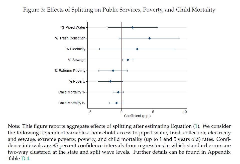
However, the expansion does show up in services. Trash collection rises 4.4%, sewage 1%. Piped water and electricity do not show any significant change. This should not be interpreted as a minor result or an econometric kink, because trash collection and primary education are exclusively municipal mandates, while water, sanitation, and electricity are shared with state and federal governments. When accountability is shared, no level of government takes ownership, and investment falls between the cracks (Kresch, 2020).
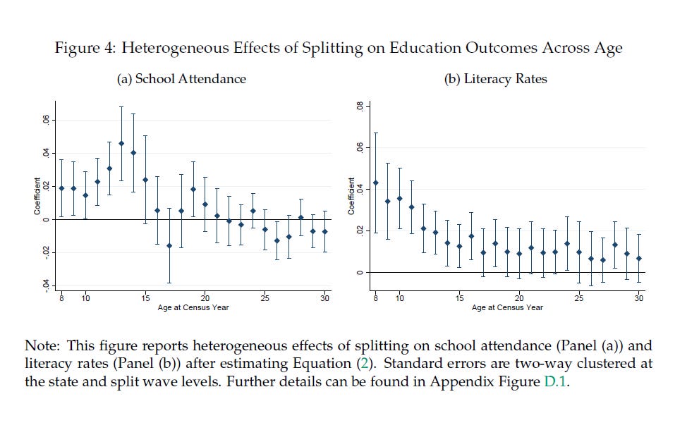
For education, they use a different identification strategy. The authors borrow the cohort exposure logic from Duflo (2001) on Indonesian school construction. If splitting builds out schooling infrastructure, the cohorts young enough to use the new schools should show the biggest gains. They formalize this as:
where i indexes individuals, k indexes age at the census year, m and s index municipality and state, and t indexes census year. The fixed effects α_km and α_kt absorb baseline differences across age-municipality and age-time cells. The coefficient β_τ on the interaction of split status and age dummy identifies the differential effect of splitting on cohort τ relative to the omitted age category, comparing split and almost-split municipalities before and after.
The results trace out an exposure gradient. Kids under fifteen in the post-split census show literacy gains up to four percentage points and school attendance gains up to five. Older cohorts, who had already cycled through, see much smaller effects. The crowding-out tells a coherent story. Nonprofit jobs in education shrink while public-sector jobs in education expand. Splitting reorganizes the supply of schooling from third-sector provision toward direct municipal provision.
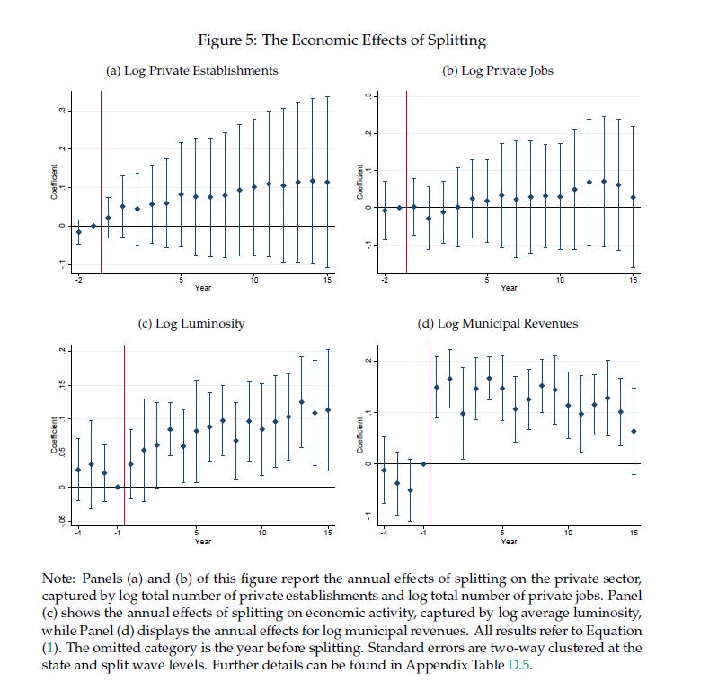
When we go beyond the public sector, however, the story gets murkier. Private-sector jobs and establishments tick up, but the confidence intervals are wide. Retail and services drive most of the new establishments, but agriculture, manufacturing, and construction barely move. Nighttime luminosity, validated as a proxy for local GDP by Henderson, Storeygard, and Weil (2012) and Henderson, Squires, Storeygard, and Weil (2018), rises sharply for five years and stabilizes at 8% above the counterfactual. Because household access to electricity does not change, the luminosity increase is not just something like streetlights or bonfires.
Cui bono?
Here is the result that should change how people read the rest of the paper. Within each new municipality, there are typically three kinds of districts:
i) the applicant district that initiated the split,
ii) sometimes other peripheral districts that came along (the "remaining" districts),
iii) and the headquarters district of the original parent municipality.
The luminosity gains are not spread evenly across them. They are concentrated almost entirely in the applicants.
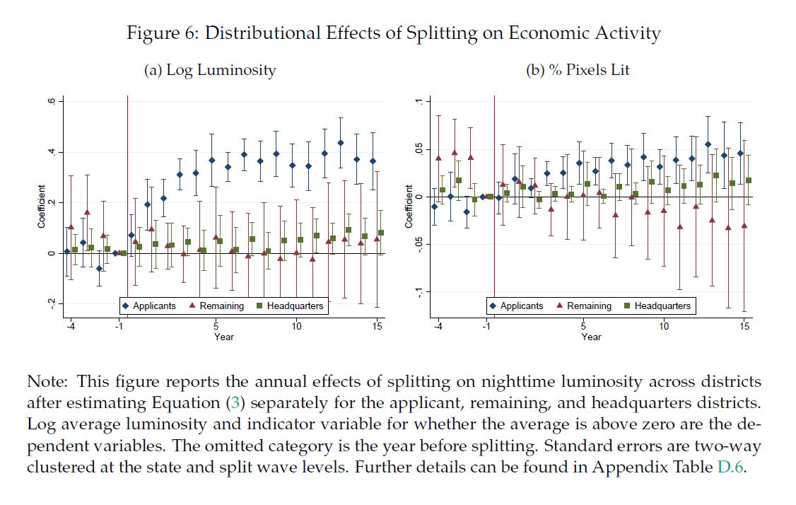
The applicants’ luminosity rises about 34 log points (40%) over 15 years. The remaining districts show no detectable change. The old headquarters districts pick up a small gain of around six percent. The extensive-margin measure (the share of pixels lit) tracks the intensive measure. It rises about four log points in applicants and barely moves elsewhere. Measuring luminosity outside a 5km radius of the new town hall, to test whether the gains are concentrated around the seat of government as in Bluhm, Lessmann, and Schaudt (2023), gives essentially the same estimate. The growth is spread across the applicant district, not concentrated in the new political center.
Table 3 unpacks the heterogeneity. The benchmark coefficient on log luminosity for applicant districts is 0.35. Interacting that coefficient with baseline characteristics shows where it comes from. The gain is larger in districts with lower baseline urbanization (the interaction coefficient is −0.01 per percentage point of baseline urbanization, significant at one percent), larger in districts further from the old town hall (the interaction with log distance is positive at 0.24), and somewhat larger in districts further from the state capital. The interaction with the baseline population is statistically insignificant. The interaction with district area is negative and significant at −0.13, meaning the per-district gain is larger when the new municipality is geographically smaller.
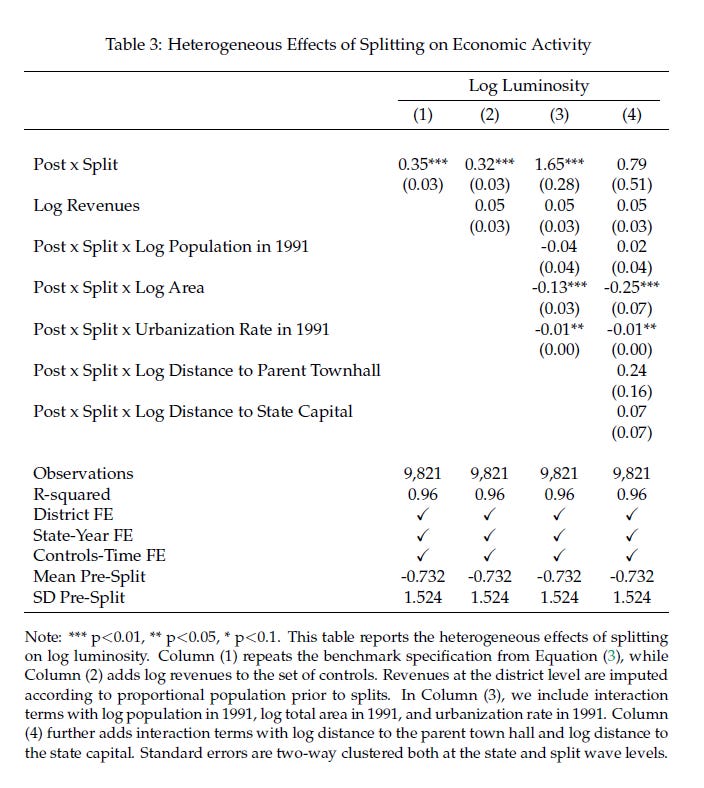
This heterogeneity is one of the key results of this paper. A pure income shock would raise every component of the municipality's spending in proportion to the size of the shock. What we see instead are tracks distance from the old town hall and low urbanization, which are precisely the proxies for capture and neglect by the parent government identified by Mansuri and Rao (2012) in their survey of decentralization in the developing world. The gains are largest in the districts that were structurally worst served before the split. In other words, we see that the improvement in participation and constituents’ voices truly matters for local development.
Money Versus Power
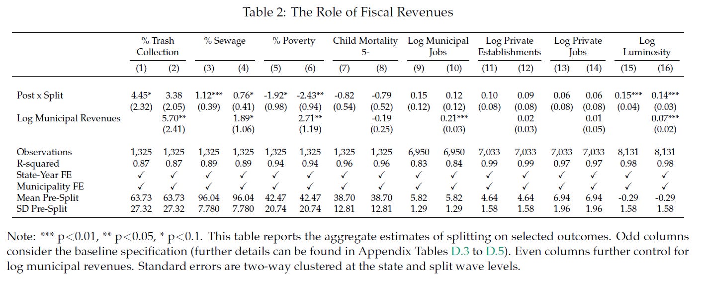
The temptation, once you see the revenue numbers, is to attribute everything to federal transfers. Total municipal revenues jump 15% after a split, almost entirely from federal transfers, which is, naturally, a real shock, and it explains part of the result. But only a part.
Dahis and Szerman (2025) test the proposition directly with a horse race. The benchmark specification on outcome y is re-estimated controlling for log municipal revenues:
If the gains were just an income effect, β would shrink toward zero once revenues are absorbed. It shrinks, but it lingers as a substantively large and significant effect across outcomes. For trash collection, the coefficient drops from 4.45 to 3.38 percentage points. For sewage, from 1.12 to 0.76 percentage points. For luminosity (in a parallel district-level horse race using imputed district revenues), from 0.35 to 0.32 log points. Income explains a slice of the result. It does not explain most of it.
The asymmetric service pattern is the more persuasive piece of evidence. Gains show up where new municipalities have unilateral authority and vanish where they share authority with higher levels of government. A pure cash injection would not behave that way, and the geographic heterogeneity points in the same direction. And after splitting, applicant and headquarters districts elect mayors from different parties about 75% of the time, rising to 85% two decades later. The applicants were not politically aligned with their old headquarters. They had distinct preferences and, once they could express those preferences in their own elections, they did. This is the premise of Oates (1972) tested literally, in line with the formal representation logic of Persson and Tabellini (2002) and the accountability mechanism of Seabright (1996).
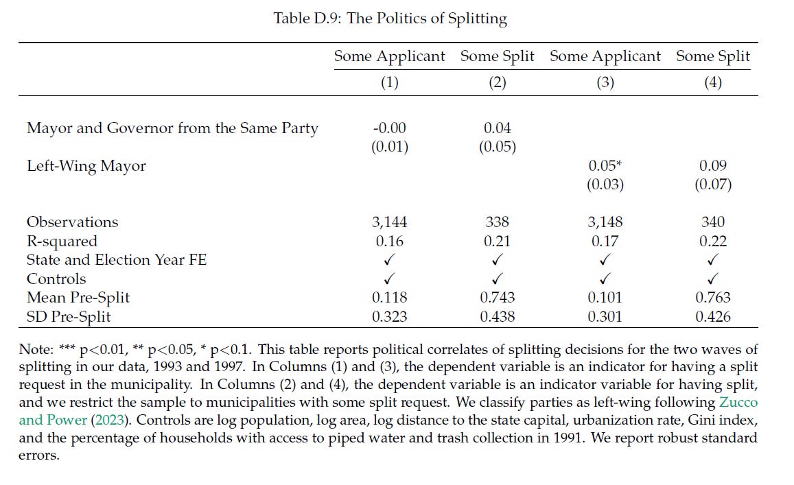
The political-economy alternatives mostly do not fit. Hassan (2016) and Gottlieb, Grossman, Larreguy, and Marx (2019) model splitting as an endogenous distributive choice by incumbent politicians who benefit from carving away opposition voters. The Brazilian data show no such pattern. Political alignment between local mayors and state governors does not predict either the filing of split requests or their success (Appendix Table D.9 of Dahis and Szerman 2025). Left-wing mayors are somewhat more likely to file split requests but no more likely to succeed. The boom does not look like a state-level partisan project.
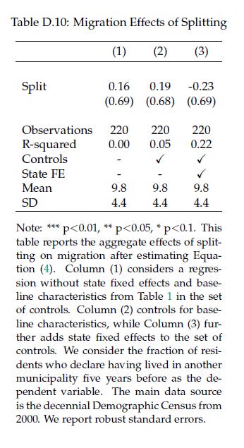
Tiebout-style migration also fails to show up. A cross-sectional regression using the 2000 census, which is the first to record municipality-of-residence five years earlier, finds no effect of splitting on inward migration (Appendix Table D.10 of the same paper). People did not vote with their feet for the new municipalities. Whatever was driving the gains, it was not residents reshuffling across jurisdictions in search of better services. The Tiebout (1956) mechanism is absent from this case, while the Oates (1972) mechanism of better-aligned local policy is doing real work.
Does the Rest of the Country Pay
The FPM is zero-sum within each state. When new municipalities draw their share, the municipalities that did not split lose a bit of theirs. Dahis and Szerman (2025) take this seriously and run a state-level analysis. States with more splits lose more transfers, so if the policy creates losers, we should see them concentrated in high-fragmentation states. The data is clean enough to compute the share losses precisely within their sample period. Municipalities that split increased their share of federal transfers by about 20.3% on average. Municipalities that did not split saw their share fall by about 13.7% on average. The mechanical redistribution is large.
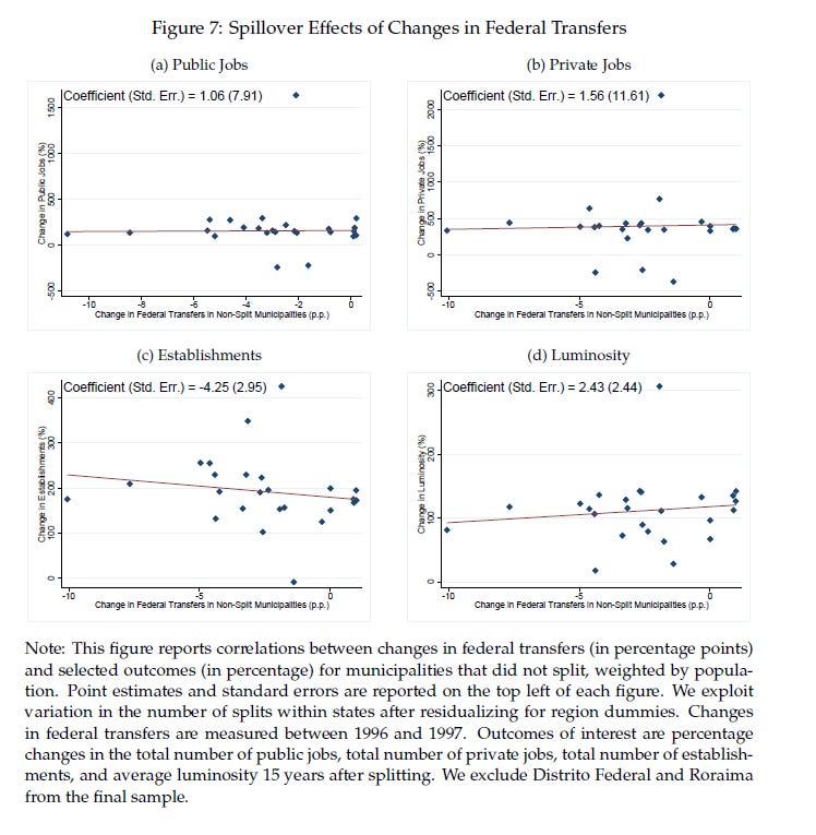
What happens to the non-splitters? The slopes from a state-level binned scatter, weighted by population and residualized for region dummies, are essentially flat. The coefficient on public jobs is 1.06, with a standard error of 7.91. On private jobs, 1.56 (s.e. 11.61). On establishments, −4.25 (s.e. 2.95). On luminosity, 2.43 (s.e. 2.44). None of these moves systematically with the size of the transfer loss. The confidence intervals are wide enough to rule out very large negative effects but not modest ones. With 25 effective states, the inference is genuinely limited, but the population coverage is essentially complete, which weakens the standard amostral critique.
The most plausible reading borrows from Liebman and Mahoney’s (2017) work on year-end federal procurement and the marginal value of public spending. Liebman and Mahoney document that federal agencies systematically spend down their budgets in the last weeks of the fiscal year on lower-value projects to avoid future budget cuts. The implication is that the marginal value of public spending can sit well below the social cost of funds in many institutional contexts. If pre-split parent municipalities looked like Liebman-Mahoney federal agencies, then reallocating FPM toward smaller new municipalities (where the marginal dollar bought more) raised aggregate welfare even at constant transfers. This is not directly tested. It is consistent with what we see.
The authors are duly cautious. The reader who wants to insist the boom was a net loss can find room to do so in the wide confidence bands, but they will have to find that room somewhere other than the data on visible economic damage to non-splits, because the data on visible economic damage is clean and shows none.
How Much of a Deal Is This
Two summary statistics tell you whether the magnitudes are large. The first is the cost per public job. The aggregate effect of splitting on municipal employment is roughly 15.8% against a baseline of 604 jobs in the year before splitting, so 95.65 additional jobs per municipality. The aggregate effect on FPM transfers is 36.75%. Translating to constant 1998 reais at 2016 dollar equivalents (the convention used by Corbi, Papaioannou, and Surico (2019) to make their numbers comparable), the additional FPM is about US$ 347,738 per municipality per year. That gives a cost per public job of around US$ 3,635 per year.
Corbi, Papaioannou, and Surico (2019) estimated US$ 8,000 per job for the same outcome from FPM transfers without an accompanying split. Splitting produces public-sector employment at roughly half the cost per dollar of transfer. For reference, Gerard, Naritomi, and Silva (2024) report a cost per job of US$ 9,799 for the Bolsa Família cash transfer program in Brazil, so splitting also dominates cash transfers on this margin.
The second statistic is the implied output multiplier. With no municipal GDP data before 2002, the authors estimate the GDP gain indirectly through the elasticity of nighttime luminosity to GDP in their sample. The luminosity gains imply about US$ 717,164 in additional GDP per municipality per year. Dividing by the US$ 347,738 in additional FPM gives an output multiplier of 2.06.
An alternative methodology from Chodorow-Reich (2019) ties the output multiplier to the employment multiplier through the production function:
where (1 − ξ) is the labor share in production, (1 + χ) is the elasticity of hours per worker to total employment, Y/E is output per worker, and μ_E is the employment multiplier (the inverse of cost per job). Using the same parameter calibration as Corbi, Papaioannou, and Surico (2019) of (1 − ξ) = 0.666, χ = 0.12, Y/E = 21,152, the splitting employment multiplier translates into an output multiplier of 4.34.
The question is that Chodorow-Reich (2019) surveys fiscal spending multipliers across mostly rich-country studies and reports a median of 1.9, but Brazilian splitting comes out at the upper end of that distribution. The interpretation is that splitting combines a transfer (which has its own multiplier) with an institutional change (which raises the productivity of the transfer). The fact that the splitting multiplier exceeds the pure transfer multiplier from Corbi, Papaioannou, and Surico (2019), which ranged from 1.1 to 2.6, is the headline summary measure of how much extra economic activity the institutional change is producing. The institutional component cannot be a null contribution if the combined multiplier is larger than the pure-transfer multiplier.
Now, none of this tells you the optimal number of Brazilian municipalities. A multiplier above the literature median says the marginal real was put to productive use during this particular boom, but it does not mean at all that further fragmentation would have the same results. The benefits Dahis and Szerman (2025) document apply to a specific configuration of unusually large pre-existing municipalities, demonstrably underserved peripheral populations, lenient state-level rules, generous federal transfers, and voluntary applications from below. Strip those conditions out and, well, everything changes.
The limitations of the paper
The textbook fiscal critique of fragmentation, that small new units cannot finance themselves, that they survive only on transfers, that the transfers impoverish the rest of the country, that the new units do not deliver services worth the money, does not survive the Brazilian data. New municipalities funded themselves through federal transfers, built bureaucratic capacity quickly, expanded the services they were uniquely accountable for, attracted private retail activity, and grew their local economies.
The municipalities that did not split do not show visible damage. The structural gradient of the gains, concentrated in peripheral low-urbanization districts far from the old town hall, fits the decentralization theory of Oates (1972) and Bardhan (2002) better than it fits any pure income-effect alternative.
The harder questions are still open. Revenue windfalls in Brazilian municipalities have been linked to higher corruption and worse politician quality (Brollo, Nannicini, Perotti, and Tabellini 2013, Boffa, Piolatto, and Ponzetto 2016). Small jurisdictions can fail to coordinate on pollution, infrastructure, and regional planning (Lipscomb and Mobarak 2017).
Nothing in the Dahis and Szerman (2025) data speaks to these costs directly, however. The aggregate question of whether Brazil should have fragmented more or consolidated requires evidence that goes beyond this paper. Recent work by Narasimhan and Weaver (2024) on splits in Uttar Pradesh and by Cohen (2022) on Uganda gives slightly different readings in those settings, which suggests that the conditions that made Brazilian splitting productive are not universal.
In a country with very large municipalities and visible peripheral neglect, subsidized voluntary splitting generated durable gains for the seceding peripheries, did not visibly drain the rest of the country, and produced new public employment at a cost per dollar that beats most fiscal interventions in the literature. The Brazilian boom is one careful data point on a long-running argument. It is worth taking seriously.
Unfortunately, Substack doesn’t allow for LaTeX in the main text, so I would like to apologize to the reader in advance for the bad formatting